Automated Coverage Analysis and Augmenting Our Understanding

Coverage analysis lets you see what happened; automated coverage analysis is about turning runtime data into insights about the code you’re testing with less manual effort.

Today we’re finishing our three-part series on code coverage by exploring this powerful approach that has applications in testing, development, reverse-engineering (RE), and fuzz testing.

• Part 1: Code coverage explained
• Part 2: 5 ways to get coverage from a binary
• Part 3: Automated coverage analysis techniques (this post)

Why automated coverage #

Most people use coverage data for two things: overall coverage metrics and manual coverage exploration.

Most people are missing out! …But not you ;)

The basic coverage metric is typically generated in an automated way, but usually the only information shown is aggregate percentages about which code is covered or not.

Manual coverage exploration, whether via lcov-style source highlighting or binary block highlighting with an RE framework like Binary Ninja, are useful because they allow you to think about why a block was covered and allow you to derive understanding based on the answer.

So if you’re used to a coverage tool like lighthouse (an inspiration for bncov, before they had Binary Ninja support) why would you be interested in automated coverage analysis? I’ll give you three reasons:

1. Automated workflows: You often ask the same questions every time you gather coverage (like in fuzzing), and just want the answers without manual effort
2. Combining analysis: You want to combine coverage data with other analysis data
3. Scripting and advanced visualizations: You want to manipulate or visualize coverage data beyond what’s currently available in a GUI

For all three of these things you need a way to programmatically access and manipulate coverage data, which is why I wrote bncov

Automated coverage workflows #

The initial motivation for bncov was to enable automated fuzz testing workflows, because any time you want to understand what the fuzzer actually exercised, block/line coverage is usually the easiest place to start.

We can start with a straightforward workflow:

1. Fuzz target and generate a corpus of inputs: afl-fuzz -i inputs -o outputs -- ./instrumented_target @@
2. Collect coverage information by executing each of the generated inputs: ~/bncov/dr_block_coverage.py outputs/default/queue -- ./uninstrumented_target @@
3. Visualize or otherwise present coverage information about the fuzz testing (e.g. open uninstrumented_target in Binary Ninja and import outputs/default/queue-cov via bncov’s context menu)

bncov allows you to import coverage data and see aggregate in a “reverse heat map” coloring scheme: blocks that are covered by a smaller percentage of the inputs are “rare” and thus are more interesting, so we color them red. More common blocks are blue, and the shades of purple are the in-between.

But we can automate more than just coloring blocks!

Common fuzzing questions and answers #

Since Binary Ninja gives us a lot of static analysis information on the target, we can leverage this to answer common questions about fuzz testing, like:

1. Was my fuzz testing successful (did it work)?
   • A decent approach would be to compare how many functions the initial input covered to the number of total functions covered by the aggregate. Effective fuzz testing should discover many more new blocks and functions compared to a single starting input.
2. Where in the code did fuzzing stop? (related: “what did I miss?”)
   • We can look at the “coverage frontier”, any place where a conditional jump has at least one outgoing edges that isn’t covered. Useful for understanding which conditionals may either have complex or precise requirements on input, OR places where the control flow isn’t affected by the input
3. Did any sensitive or dangerous functions get called?
   • It’s common to check the coverage for calls to sensitive or dangerous functions (strncat, system, etc) to see if fuzz testing was able to reach them. To see the contents of the arguments to such calls you might switch to a debugger, but coverage analysis can be a great filter to downselect the inputs you want to dive deeper on. Scripting’s flexibility allows you to create compound conditions like “Show inputs that cover the functions login and getUserPrivateData but not checkPassword”.

Similar analysis could be applied to testing and RE, but the implementation will depend on the use case.

This seems to be an under-explored topic, so please let me know if you find something out there or come up with something yourself that works!

Combining other analysis data with coverage #

While automating workflows typically involves combining specific kinds of analysis data (specifically static analysis data from Binary Ninja), there’s really no limit to what you can do.

To me, block coverage data is the perfect bridge between dynamic and static analysis data: it is among the least expensive dynamic information to collect and store, but it can link data gathered during execution with practically any other data you can think of.

One of the simplest static analysis measures is cyclomatic complexity. It’s an interesting metric because high cyclomatic complexity means a function has many potential paths through it, which means it’s typically harder to reason about and harder to test exhaustively (which suggests the function might also contain bugs).

In fuzz testing, we’re often interested in high cyclomatic complexity functions because it’s usually easier to get coverage on the different paths by generating inputs with a fuzzer than it is writing unit tests manually.

If you want to target high cyclomatic complexity functions, but you may not want to harness them directly; rather you’d want to find a function that makes sense to target that also reaches a lot of complexity. By pairing the complexity of each function with a call graph, you can calculate exactly this, which I call “descendent complexity” (analysis I first described in my ShmooCon 2020 talk) which is an analysis included in Ariadne.

The following graph from Ariadne shows a motivating example from my talk (around 37:00), where at the time someone only harnessed the function tjDecompress2; missing a decent amount of complexity related to YUV handling. Using this kind of visualization where nodes are sized based on complexity, it is immediately clear that both tjDecompress and tjDecompressToYUV might be interesting to target with fuzzing, which is exactly what the dependendent complexity metric would suggest.

You can then repeat this analysis and combine data after each successive round of harness creation and fuzz testing to determine what code remains uncovered and what the next best thing to target would be. You can even set this up as an automated workflow!

Complexity is just one metric though; you could use any other interesting analysis to focus your efforts: xrefs to dangerous functions, findings from static analysis tools, presence of stack buffers or malloc/free calls… whatever you like.

Advanced Visualization #

The image from the last section was an obvious preview; I’m wouldn’t be satisfied talking about numbers around things like descendent complexity and coverage… this is something that just makes sense when you have a visualization, and that’s where Ariadne comes in.

While I wrote about Ariadne in a previous post, the upshot is that it pairs some basic static analysis with a graph helper, and it’s intended to be used in two ways: interactively and programmatically.

First, as an interactive tool, it allows you to see and explore the code as you navigate around in Binary Ninja, seeing the local neighborhood of the call graph as well as function complexity and coverage (if you import coverage from bncov).

But as a scriptable tool, it gives you the ability to get an interactive visualization of arbitrary function graphs.

Some basic workflows like source/sink analysis come built in, but since Ariadne uses the well-known Python library networkx ( docs) to construct and manipulate graphs, it’s easy to construct arbitrary function graphs and see the picture of anything you want.

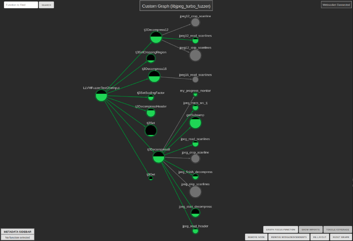
For example, let’s say we want to see the coverage of a fuzz target, plus the functions that are immediately reachable but didn’t get covered.

First we open the target in Binary Ninja, import the coverage files with bncov, analyze the target with Ariadne, and then in the interactive scripting console of Binary Ninja:

import networkx as nx
import bncov
import ariadne

covdb = bncov.get_covdb(bv)
covered_func_starts = covdb.get_functions_from_blocks(covdb.total_coverage)
covered_funcs = set([bv.get_function_at(addr) for addr in covered_func_starts])
uncovered_funcs = set()
for func in covered_funcs:
    for child in func.callees:
        if child not in covered_funcs:
            uncovered_funcs.add(child)

funcs_to_graph = covered_funcs.union(uncovered_funcs)
callgraph = ariadne.core.targets[bv].get_callgraph()
subgraph = nx.subgraph(callgraph, funcs_to_graph)
ariadne.core.push_new_graph(subgraph)

Running this on a CTF-sized target gives us a visualization we can look at in a browser that we can start to wrap our heads around… but even this is still a bit much; you don’t want too large of a graph to start.

We can infer a few things just starting out, like there are some edges in the callgraph that Binja didn’t pick up, but we can just focus on the largest connected component to filter those out. There’s also some heap wrapper functions we can quickly remove with the graph controls to clean up the picture a little.

largest_component = max(nx.connected_components(subgraph.to_undirected()), key=len)
new_subgraph = nx.subgraph(subgraph, largest_component)
ariadne.core.push_new_graph(new_subgraph)

Having something like this really helps us understand exactly what functions got covered (and how much, judging by the fill levels of the covered functions), which is a pretty powerful tool for understanding coverage.

And just like that, a small amount of scripting has turned our seemingly boring coverage data into a sweet custom visualization!

Coverage covered #

Whew, so this the end of a three-part series where we talked about what code coverage is, some ways to get coverage data, and some of the more interesting applications of coverage analysis, particularly with regards to automated/scripted analysis and visualization.

Hopefully this helped fill in the gaps on what coverage is and how it can help in a variety of applications, from RE to code testing.

If you’ve applied bncov or Ariadne to any of your own workflows, or even just made a cool screenshot or picture you thought helped you understand something, please drop me a line on Twitter or any other of my socials! Til next time, keep your codebases… covered?